[1]:
import numpy as np

import matplotlib.pyplot as plt

from neurodsp.sim import sim_oscillation
from neurodsp.spectral import compute_spectrum

from timescales.sim import sim_ar
from timescales.fit import ARPSD, PSD
from timescales.autoreg import compute_ar_spectrum
from timescales.plts import set_default_rc
set_default_rc()
02. PSD Objects#
This tutorials explores the use of the PSD objects. There are two PSD models available:
ARPSD: exact, derived from AR(1)PSD: approximate
[2]:
# Settings
n_seconds = 20
fs = 1000
phi = 0.95
tau = -1 / (np.log(phi) * fs)

# Simulate a signal
np.random.seed(0)
sig = sim_ar(n_seconds, fs, phi)
sig += sim_oscillation(n_seconds, fs, 10) * 5
Compute Spectra#
PSD objects have a .compute_spectrum method that may be called from an empty intialization. This method supports neurodsp’s compute_spectrum, or timescale’s compute_ar_spectrum function if ar_order is passed. External functions that compute spectra may be used, and these arrays may be specificed when initalizing a PSD object. Once the freqs and powers attributes have been defined, the model may be fit.
[3]:
# Compute spectrum using external function
psd = PSD()
freqs, powers = compute_spectrum(sig, fs)
psd = PSD(freqs, powers)

# Or using class method
psd = PSD()
psd.compute_spectrum(sig, fs)
Fitting: 1d#
PSD objects support FOOOF models or any loss function supported by scipy.optimize.least_squares. If a loss function is specified, a single call to scipy’s curve fit is used to robustly optimize the aperiodic Lorentzian model.
When method kwarg is in ["fooof", "huber", ... scipy_loss_fn]:
When method='ar':
Alternatively, ARPSD objects optimize more complex forms. Below \(k\) is the AR order, for exat models this should be one. When AR(1) models do not suffice, the order may be raised, e.g. AR(p=10).
[4]:
%%timeit
# Using the fooof package
psd.fit(method='fooof', fooof_init={'peak_threshold': 2.5})
10.8 ms ± 220 µs per loop (mean ± std. dev. of 7 runs, 100 loops each)
[5]:
%%timeit
# Using fooof aperiodic model + robust regression
psd.fit(method='huber')
2.93 ms ± 47.7 µs per loop (mean ± std. dev. of 7 runs, 100 loops each)
[6]:
%%timeit
# Using AR(1)-PSD model + robust regression
psd.fit(method='ar')
1.79 ms ± 22.8 µs per loop (mean ± std. dev. of 7 runs, 1,000 loops each)
[7]:
psd.plot()
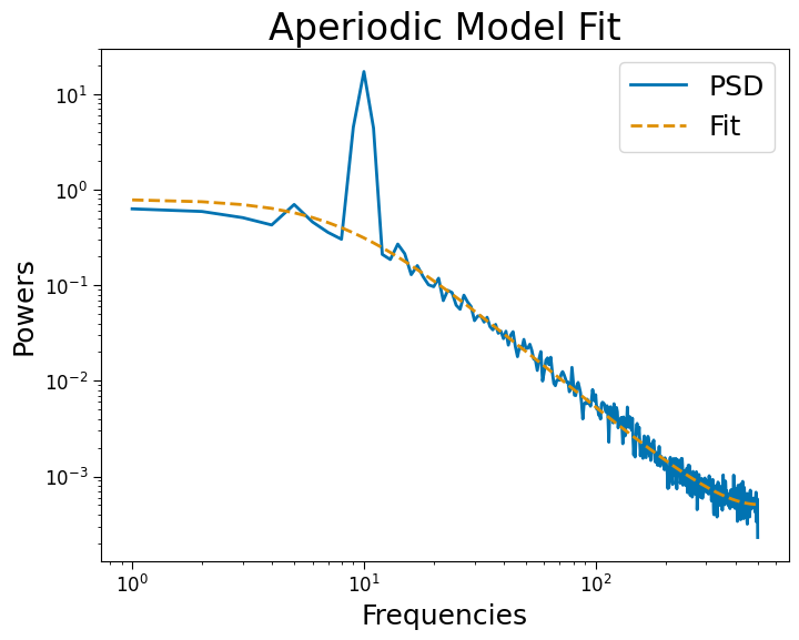
Fitting: 2d#
2d arrays of signals or powers are supported.
[8]:
# Simulate signals
fs = 1000
n_seconds = 5

nsigs = 20

sigs = np.zeros((nsigs, int(n_seconds * fs)))
osc = sim_oscillation(n_seconds, fs, 10) * 5
for ind in range(nsigs):
    np.random.seed(ind)
    sigs[ind] = sim_ar(n_seconds, fs, phi)
    sigs[ind] += osc
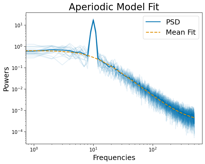
[9]:
# Fit AR(1)-PSD robustly
psd_ar = PSD()
psd_ar.compute_spectrum(sigs, fs, n_jobs=-1)
psd_ar.fit(method='ar')
psd_ar.plot()

[10]:
# Fit FOOOF robustly
psd_robust = PSD()
psd_robust.compute_spectrum(sigs, fs, n_jobs=-1)
psd_robust.fit(method='huber')
psd_robust.plot()
Results#
Optimized parameters, labels, and model r-squared values are stored as attributes.
AR(1)-PSD model:
[11]:
psd_ar.param_names
[11]:
['phi_0', 'offset']
[12]:
psd_ar.params[:5] # 'phi_0', 'offset'
[12]:
array([[0.94332773, 0.00179388],
       [0.95363645, 0.00189638],
       [0.95659961, 0.00195419],
       [0.94777176, 0.00182976],
       [0.94924305, 0.00177143]])
[13]:
psd_ar.tau[:5] # timescales
[13]:
array([0.01714045, 0.02106471, 0.02253757, 0.01864226, 0.01919739])
[14]:
psd_ar.rsq[:5] # r-squared
[14]:
array([0.91003531, 0.91156543, 0.91498511, 0.91001191, 0.91090734])
FOOOF model with robust regression:
[15]:
psd_robust.param_names
[15]:
['offset', 'knee_freq', 'exp', 'const']
[16]:
psd_robust.params[:5]
[16]:
array([[2.06682305e+00, 1.29289216e+01, 2.20366300e+00, 3.30445219e-04],
       [1.97265076e+00, 1.00588562e+01, 2.13388043e+00, 2.87552714e-04],
       [1.73676892e+00, 7.20600236e+00, 2.00725277e+00, 2.45701097e-04],
       [2.03090920e+00, 1.13857241e+01, 2.18318743e+00, 3.41204660e-04],
       [1.60177883e+00, 7.70251629e+00, 1.96763137e+00, 2.27468325e-04]])
[17]:
psd_robust.rsq[:5]
[17]:
array([0.91065383, 0.91134276, 0.91532763, 0.91052842, 0.9111365 ])
[18]:
psd_robust.tau[:5]
[18]:
array([0.01230999, 0.01582237, 0.02208644, 0.01397846, 0.02066272])