import numpy as np
from tqdm.notebook import tqdm

from neurodsp.sim import sim_oscillation, sim_powerlaw
from neurodsp.filt import filter_signal
from neurodsp.spectral import compute_spectrum

from fooof import FOOOF
from bycycle import Bycycle

from ndspflow.workflows.workflow import WorkFlow

WorkFlow Class

WorkFlow objects wrap analyses that are typically functionally oriented into a unified object. This provides reproducible analyses, a unified interface for a variety of DSP packages and models, and memory/computational efficiency. This class consist of three types of nodes:

1. Input : Defines the raw input numpy array, including simulations, reading BIDS structure, or custom classes or functions to read in raw binary data.

2. Transformations : Defines the order of preprocessing operations used to manipulate the raw array input. Any function that accepts an y-array, and returns an y-array, with or without an x-array, are supported. This allows interfacing of signal processing packages, such as scipy, numpy, mne, neurodsp, etc. Examples: filtering, re-referencing, ICA, frequency domain transformations, etc.

3. Models : Defines the model class that is used to fit or extract values out of the transformed array. Models should be initialized and contain a fit method that accepts array definitions. Examples: fooof, bycycle.

Forks : Forks refer to the splitting of the workflow into multiple streams. Forks may optionally have additional transforms (e.g. one model may want power spectra, whereas another requires time series).

Initialization

When initializing a WorkFlow object, arbitary keyword arguments may be passed that are required by one of its sub-classes. In the case below, we want to set the seeds attributes, required by the Simulation sub-class accesed via the .simulate() method. X-axis values may be optionally defined here, if required by the model passed to the .fit() method.

# Settings
n_seconds = 10
fs = 1000
seeds = np.arange(4)

# Initialize
wf = WorkFlow(seeds=seeds)

1. Input

Next we define the input array, here a series of simulations. Multiple simulations calls may be stacked to create the input array. Any simulation function may be used as long as a single array is returned. The way arrays are combined are defined by the operator argument. The general form follows:

.simulate(func, *args, operator, **kwargs)

# 1. Define np.array input
wf.simulate(sim_powerlaw, n_seconds, fs, exponent=-2)
wf.simulate(sim_oscillation, n_seconds, fs, freq=10, operator='add')
wf.simulate(sim_oscillation, n_seconds, fs, freq=20, operator='add')

2. Transform

The input array may transformed using any function, as long as a single array is returned. Transformation calls may also be stacked to define a series of transformations (e.g. pre-processing steps). The axis argument is used for ndarrays with greater than two dimensions and specifies which axis to iterate over to apply the transform. The general form follows:

.transform(func, *args, axis=None, **kwargs).

# 2. Transform input
wf.transform(filter_signal, fs, 'lowpass', 300, remove_edges=False)

3. Model

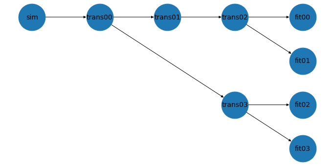
Up to this point, all sub-workflows share the same set of simulations (4 unique seeds) and the 300 Hz low-pass filter. The .fork(index) method is used to split the workflow into sub-workflows. The first .fork(0) called with a unique index argument creates a save state at the point of the call. Subsequent .fork(0) calls restore that state at the time of the inital .fork call before proceding. New fork calls (e.g. .fork(1)) creates a new save state that can be later restored upon subsequent calls of .fork(1). In general, a unique index passed to .fork(ind) creates a new save state, and an existing index restores the corresponding save state at the time of the first call. Below, we fork the workflow into sub-flows that end on two sets of FOOOF and Bycycle models. Note that the .fit() calls belows does not run the workflow and instead adds fitting the model to the call stack. Once the WorkFlow is complete, the .run() method is used to execute the workflow, as shown in the next section.

# Create a fork that references the transform in the previous cell
wf.fork(0)

# All FOOOF sub-workflows share these transformations
wf.transform(filter_signal, fs, 'lowpass', 200, remove_edges=False)
wf.transform(compute_spectrum, fs)

# FOOOF sub-workflows
wf.fork(1)
wf.fit(FOOOF(verbose=False, max_n_peaks=2), (1, 100))

wf.fork(1)
wf.fit(FOOOF(verbose=False, max_n_peaks=2), (1, 200))

# Restore that state after the first filter, two code cells above
wf.fork(0)

# All Bycycle sub-workflows  share these transformations
wf.transform(filter_signal, fs, 'lowpass', 100, remove_edges=False)

# Bycycle sub-workflows
wf.fork(2)
wf.fit(Bycycle(), fs, (1, 100))

wf.fork(2)
wf.fit(Bycycle(), fs, (1, 200))

# Plot the workflow
wf.plot()

Execute

Lastly, the WorkFlow is executed in parallel using the run method. Results are accesible via the .results attirbute. The order of models in .results maintains the in the same order as the WorkFlow was defined. Here the first index of .results refers to the simulation seed (in order of seeds above) and the second index refers to the order of the .fit calls above.

# Execute workflow
wf.run(n_jobs=1)

# Access results
wf.results

array([[<fooof.objs.fit.FOOOF object at 0x7fb6e6b89400>,
        <fooof.objs.fit.FOOOF object at 0x7fb6e6b89940>,
        <bycycle.objs.fit.Bycycle object at 0x7fb6e6b89e50>,
        <bycycle.objs.fit.Bycycle object at 0x7fb6e6b92400>],
       [<fooof.objs.fit.FOOOF object at 0x7fb6e6b89700>,
        <fooof.objs.fit.FOOOF object at 0x7fb6e6b92280>,
        <bycycle.objs.fit.Bycycle object at 0x7fb6e6b92a30>,
        <bycycle.objs.fit.Bycycle object at 0x7fb6e6b92c70>],
       [<fooof.objs.fit.FOOOF object at 0x7fb6e6b89790>,
        <fooof.objs.fit.FOOOF object at 0x7fb6e6b92af0>,
        <bycycle.objs.fit.Bycycle object at 0x7fb6e6b92fd0>,
        <bycycle.objs.fit.Bycycle object at 0x7fb72dccd250>],
       [<fooof.objs.fit.FOOOF object at 0x7fb6e6b899d0>,
        <fooof.objs.fit.FOOOF object at 0x7fb72dccd0d0>,
        <bycycle.objs.fit.Bycycle object at 0x7fb72dccd5b0>,
        <bycycle.objs.fit.Bycycle object at 0x7fb72dccd7f0>]],
      dtype=object)

Returning Model Attributes

The the return_attrs arguments is used to transfer any attribute in the model class (here a FOOOF and Bycycle object) to the results attribute of the WorkFlow class. This is more memory efficienct as copies of PSDs, time series, and all other model class attributes are not passed to the results attribute and are dropped from memory.

If return_attrs is a string or list of strings, these attribues are expected to exist in each model. A 2d list of return_attrs strings provides the greatest flexibility, pairing each list of attributes to each model.

# Execute workflow
attrs = [
    *[['peak_params_', 'aperiodic_params_', 'r_squared_']] * 2, # FOOOF attributes
    *[['time_peak', 'time_rdsym', 'monotonicity']] * 2          # Bycycle attributes
]

# Rerun the workflow
wf.run(attrs=attrs)

wf.results[0][0]

{'peak_params_': array([[10.00966989,  3.32493202,  1.9312485 ],
        [19.99507858,  4.0559911 ,  1.99129882]]),
 'aperiodic_params_': array([-1.20772038,  1.96193711]),
 'r_squared_': 0.97146685302719}